In my last article, I wrote about interleaved and planar memory layouts, and when to use each. Both layouts can contain the exact same information using the exact same amount of memory. One consideration when choosing whether to store data in interleaved or planar layout is the types of operations that will be performed on the data. Due to the principle of locality, significant performance gains can sometimes be obtained by choosing one over the other – pixel-level operations may be faster in interleaved layout, while channel-level operations may be faster in planar layout.

To exemplify this, I published unsophisticated separable 2D convolution algorithms (for an overview of separable convolution, check out this video). The code includes a performance-testing application that performs 2D separable convolutions over the same data using both interleaved and planar memory layouts, which demonstrates that the memory layout can have a significant impact on different algorithms that perform the exact same image processing computations.

Setup

I built and ran the performance testing application on my machine, which is an older Intel NUC with an Intel i5-4250U, 8GB of RAM, and 148GB SSD. At the time of running the test, Windows 10 Pro Version 1909, Build 18363.1139 was installed.

The build directory was configured to build with Visual Studio 2019 (cl version 19.27.29111) using the command below:

"C:\Program Files (x86)\Microsoft Visual Studio\2019\Community\Common7\IDE\CommonExtensions\Microsoft\CMake\CMake\bin\cmake.exe" --no-warn-unused-cli -DCMAKE_EXPORT_COMPILE_COMMANDS:BOOL=TRUE -H<src dir> -B<build dir> -G "Visual Studio 16 2019" -T host=x64 -A x64

A release configuration of the application was built with the command below:

"C:\Program Files (x86)\Microsoft Visual Studio\2019\Community\Common7\IDE\CommonExtensions\Microsoft\CMake\CMake\bin\cmake.exe" --build <build dir> --config Release --target ALL_BUILD -- /maxcpucount:6

To obtain runtimes for the different algorithms, I closed all open applications except VS Code, then ran the following command in the VS Code Terminal window:

interleaved_vs_planar.exe 2000 3000 4 3

This command creates a 2000 x 3000 x 4 (H x W x D) float matrix filled with random values in [0, 1]. It then performs 3 iterations of each test.

Tests

The application performs 5 tests, which are explained in the README.md and summarized below.

  1. interleaved3: Interpret the data as interleaved, and perform per-channel 2D separable blur using a kernel size of 3
  2. planar3: Interpret the data as planar, and perform per-channel 2D separable blur using a kernel size of 3
  3. interleaved7: Interpret the data as interleaved, and perform per-channel 2D separable blur using a kernel size of 7
  4. planar7: Interpret the data as planar, and perform per-channel 2D separable blur using a kernel size of 7
  5. planar7withTranspose: Interpret the data as planar, and perform per-channel 2D separable blur using a kernel size of 7. However, rather than performing horizontal and vertical convolution, perform horizontal convolution, transpose, horizontal convolution again, and transpose again.

In these experiments, the interleaved tests are performed on an interleaved layout of the data, while the planar tests are performed on a planar layout of the same data. In other words, the data at a given (column, row, channel) tuple is the same whether the data is in interleaved or planar layout. For clarity, it’s important to note that the particular data values in these floating point computations should not make a significant difference in the runtime, especially because all the input and output data should be in the range of [0.0, 1.0]. However, this setup allows the results of the computations to be compared directly, so that the reviewers can be confident that the same computations are occurring.

Every iteration of a test is performed before the next test is run. Statistics for the iteration with minimal total runtime are saved for output.

Results

The results obtained on the test machine are shown below, with time values recorded in seconds:

test,horizontal,transpose,vertical,total
interleaved3,0.070904,0,0.911467,0.982371
planar3,0.0454543,0,0.653508,0.698962
interleaved7,0.129526,0,0.889743,1.01927
planar7,0.0996537,0,0.645452,0.745106
planar7withTranspose,0.0995849,0.519957,0.104595,0.724137

For ease of viewing, the data has been formatted as a table below:

testhorizontaltransposeverticaltotal
interleaved3 0.07090400.911467 0.982371
planar3 0.045454300.653508 0.698962
interleaved7 0.12952600.889743 1.01927
planar7 0.099653700.645452 0.745106
planar7withTranspose 0.0995849 0.519957 0.104595 0.724137

In the first 4 tests, there is no transpose, so the transpose time is 0 for those tests; only the planar7withTranspose test includes a transpose operation so it is the only test with a non-zero transpose time.

Discussion

There are clear trends in the data. Some were expected, while others were not expected.

Interleaved vs planar

The planar3 total time is ~71% of the interleaved3 total time. The planar7 total time is 73% of the interleaved7 total time. The vast majority of the runtime for any of these convolutions occurs in the vertical convolution, which is another demonstration of the principle of locality.

Without getting too deep into the details of memory retrieval and caching, the basic idea is that when the program requests a single float (4 bytes) from memory, the processor actually retrieves those bytes as well as quite a few more adjacent bytes (up to 60 on modern processors). This adjacent data is stored in the fastest part of the processor’s cache and is potentially orders of magnitude faster to access than the data in memory.

Thus, it’s likely that in the horizontal planar convolution, requesting the data for the first element in the matrix causes the processor to retrieve all the matrix data required for ~16 operations. After the first operation, the next ~15 incur a fraction of the memory access cost. The cycle repeats itself when the next element of matrix data that’s not in the cache is requested.

There is a similar, but smaller effect in the horizontal interleaved convolution. The implementation iterates completely over the data in a channel before moving to the next channel. This means in practice that the horizontal convolution data is essentially operating over moderately sparse data. In this case, since the depth is 4, requesting data for the first element in the matrix causes the processor to store all the matrix data for ~4 operations in its fastest cache.

In contrast to this, the vertical convolutions in each layout essentially need to access data in memory, rather than cache, for probably every operation. In a sense, in these implementations, the vertical convolution almost certainly never gets data for the next operation “for free.”

Kernel size, 3 vs. 7

When comparing the horizontal convolutions, ie interleaved3 vs. interleaved7 or planar3 vs. planar7, there is an expected significant increase in runtime. Interleaved7 horizontal runtime is ~182% of interleaved3 horizontal runtime, while planar7 horizontal runtime is ~219% of planar3 horizontal runtime. The likely explanation for this significant increase is because there are simply more computations occurring – for a kernel of size 7, each element in the convolution is a function of 7 elements, while a kernel of size 3 results in a function of 3 elements. The operation on 7 elements must therefore compute 7 multiplications and 6 additions (13 total operations), while the operation on 3 elements must compute 3 multiplications and 2 additions (5 total operations). Therefore under ideal conditions we would expect the runtime of the size 7 kernel to be 260% of the runtime of the size 3 kernel. We can conclude that the conditions in these computations are not ideal, likely due to delays retrieving the required data from memory.

However, when comparing vertical convolutions, there is a very unexpected decrease in runtime. The difference is small, but consistent between interleaved3 and interleaved7 as well as planar3 and planar7. In either case, the number of operations in the size 7 kernel computation is still 260% of the computations in the size 3 kernel computation: 13 operations compared to 5. Therefore these results indicate that the size 7 routines somehow performed far more operations slightly faster than the size 3 routines. This is despite the fact that the routines are template functions, meaning that the C++ code for the size 3 & size 7 routines was the same!

No investigation was performed to understand the cause of this unexpected result.

planar7withTranspose

After noticing that vertical convolution dominated the runtime of the separable convolution, this test was conducted to see if a transpose + horizontal convolution + transpose could be faster than a single vertical convolution. In these results, a transpose + horizontal convolution + transpose takes ~97% of the time of a single vertical convolution. Performing the operation this way was clearly faster, though the difference is marginal for this test.

Considerations

These convolution implementations are only intended to demonstrate that choosing interleaved or planar can have a significant effect on runtime, depending on the algorithm that is running. They are not sophisticated or optimized implementations of convolutions, and are not intended to show minimal convolution runtime.

These results imply that planar layout is faster than interleaved layout for convolution. However, it’s more accurate to say that planar layout can be faster than interleaved for convolution. It’s certainly possible to write optimized implementations of convolution for interleaved layout by changing the order of operations to exploit memory already in the cache. It’s also possible to obtain very significant reductions in vertical convolution runtime by changing the order of operations. However, writing these sophisticated or optimized routines can be time consuming and error prone, and could be highly implementation or even processor specific. On the other hand, it’s likely that these optimizations would yield far better runtime improvements than just translating between interleaved and planar layout.

Another method of improving convolution performance would be to use an existing optimized implementation, such as the free Intel IPP. Intel IPP provides processor-specific optimized implementations of various convolutions. Since they are free to obtain and are very permissive in their licensing, there’s almost no reason not to use them. The performance improvement obtained by using an implementation like this is almost guaranteed to dwarf any improvement gained by translating from interleaved to planar or vice-versa.

In defense of this experiment, it’s clear that the relatively simple operation of translating between interleaved and planar layout can produce significant runtime reduction. This is an important conclusion, because not every image processing algorithm has a free, optimized implementation readily available, and development schedules do not always allow developers to write sophisticated implementations of image processing algorithms. Knowing that bottleneck algorithms are channel-level or pixel-level operations could allow a developer to gain significant runtime improvement for very minimal investment in development and testing.

The unexpected result in the vertical convolution, where the runtime decreased between the size 3 and size 7 kernel, would warrant further investigation in a product environment. To identify the cause of this unexpected result, some reasonable steps might include:

  1. a code review
  2. reproduction by another team member
  3. additional experiments using different horizontal size, vertical size, depth, and number of iterations
  4. investigation into the assembly code that the compiler produced

The planar7withTranspose test could be interesting for a few reasons. First, it may be possible to perform multiple vertical operations in the transposed matrix. This would amortize the cost of the two transposes and likely result in a significant overall runtime reduction. Second, as with all implementations in this experiment, the transpose operation is not optimized. It may be simpler to write an optimized transpose, rather than an optimized vertical convolution. Third, using this technique would allow developers to maintain a single 1D convolution implementation. This may be ideal in some conditions, for example if the convolution is expected to perform operations on the edge pixels rather than just zero them out. However, performance of the “transpose-horizontal convolution-transpose” algorithm for vertical convolution should be tested using different values for horizontal and vertical size – it’s possible that different image aspect ratios could produce different performance results.

None of the tests included the time to translate from interleaved to planar layout, or vice-versa. It’s possible that total runtime of translating, operating, and translating back would be similar or even greater than the runtime of just performing the operation on the data using a suboptimal layout. However, when multiple operations that would be optimized in the same layout are being performed in series (ie blur followed by derivative), the runtime reduction in the operations due to optimal layout may be much greater than the runtime increase due to the layout translations.

Conclusion

Storing image data in interleaved vs. planar layout can have a significant effect on performance. Converting between the two layouts is a simple operation that may lead to large runtime reductions, especially when multiple operations can be performed in sequence using the same optimal layout.

Feel free to clone the github repo and perform your own experiments! If you want to share those results with me, I can be contacted at whentouseit@avitevet.com.
Alright, so you’ve got your rasterized image, and now you want to save it to a file. You want a single file to contain all the data necessary for viewing this image, so that all a person needs is the single image file and an image viewer to look at your image. How do you save the data?

Grayscale

Grayscale images are a bit simpler than color images so we’ll start there.

Number of bytes to store the image

For the moment, let’s consider only the number of bytes that would be required for the pixels in a grayscale image, without thinking about the storage layout or the metadata. Recall that typically for a grayscale image, there’s one value for each pixel. Commonly, an 8 bit value (= 1 byte) is used for a value, allowing the pixel intensity value to range between 0 and 255. A rectangular image that’s W pixels wide and H pixels in height would have WxH total pixels. For example, if your image is 100 px wide & 200 px tall, there would be 100 x 200 = 20,000 pixels total. If each pixel can be represented by 1 byte, storing this image uncompressed would require 20,000 bytes.

Metadata

So you have your 20,000 bytes representing an image that’s 100px wide x 200px high image. Or was that 200px wide x 100px tall? Or 50px wide and 400px tall? How would an image viewer know how to display the 20,000 image bytes using only the image file?

The image file must contain data about the image, which is called metadata. The metadata typically contains information such as width, height, the component colors (aka channels or separations), and much more. This metadata is stored in the image file in a section that’s separate from the image data. Different containers such as JPG, GIF, TIFF, or PNG each have different ways of storing the metadata, and each container can store different metadata. When an image viewer detects a container, it must know where and how the metadata is stored in that container, and how to read the required metadata.

Image metadata is topic worthy of a series of articles. For an idea of the scope of the topic, the TIFF tags reference (metadata in TIFF can be stored as tags) describes hundreds of well-defined tags which describe everything from the basics like width and height all the way to niche information like the host computer used during image creation. And that is only for a single image container, TIFF!

For this article, it’s enough to know that there’s metadata in the image file that describes the image data.

Which byte represents a particular pixel?

So we’ve got our 20,000 bytes of data, and we know how wide and tall the image is. But which of the 20,000 bytes represents the top left pixel? In general, which byte represents the pixel at position (x, y)?

The answer to that question lies in the storage order of the pixels. Let’s assume that the pixels are stored in row-major order – in other words, all the pixels of a row N are stored before all the elements of row N + 1. Below is an example 2×2 image containing 4 pixels. They are labeled pixel(0,0) through pixel(1,1).

pixel(0,0)pixel(0,1)
pixel(1,0)pixel(1,1)

A file saved in row-major storage would contain the pixels in the order below. Note that all the elements of the 1st row appear before all the elements of the 2nd row:

pixel(0,0)pixel(0,1)pixel(1,0)pixel(1,1)

Pixels may also be stored in column-major order, but this is very unusual in the commonly used image layouts and I won’t describe that in this article.

So if we get the image’s height and width from metadata, and we assume that it’s in row-major order with the first data value holding the top left pixel, we can re-assemble this simple image using only the image file.

Color RGB images

Color images differ from grayscale images by containing effectively one image per color. Common color schemes are RGB (ideal for screens) or CMYK (ideal for print). We’ll now consider how to store RGB images.

Number of bytes to store an RGB image

Let’s consider only the number of bytes that would be required for the pixels in an RGB image, without thinking about the storage layout or the metadata.

A color pixel can be represented using a value for each of the component colors. In an RGB pixel, there is one value for each of the red, green, and blue colors. Commonly, 8 bit (=1 byte) values are used for each of the 3 colors. Thus, 3 bytes are used for each RGB color pixel.

A rectangular image that’s W pixels wide and H pixels in height would have WxH total pixels. For example, if your image is 100 px wide & 200 px tall, there would be 100 x 200 = 20,000 pixels total. Thus, for any given image dimensions, the number of pixels is the same regardless of whether the color scheme is grayscale, RGB, or some other color scheme like CMYK. However, while each pixel in a grayscale image commonly requires 1 byte, each pixel in an RGB image commonly requires 3 bytes. Therefore, storing this image uncompressed would require 3 * 100 * 200 = 60,000 bytes.

Which bytes represent a particular pixel?

In contrast to grayscale images where 1 byte represents each pixel value, an RGB pixel commonly requires 3 bytes. Given this requirements, which bytes in an image file’s image data represent a given pixel?

Chances are that you’ve already thought of at least one of the two common methods:

  1. Interleaved: Store all the bytes for pixel N before storing the bytes for pixel N + 1
  2. Planar: Store all the bytes for color C before storing the bytes for color C + 1

Interleaved

In the interleaved storage layout, the bytes for a pixel are contiguous. In the 2×2 image below, each pixel has RGB components.

pixel(0,0)pixel(0,1)
pixel(1,0)pixel(1,1)

This data would be stored in interleaved, row-major layout like in the diagram below. The top row indicates the 0-based index of each byte. For compactness, the RGB components of pixel(x, y) are shown as xy.R, xy.G, or xy.B, respectively.

01234567891011
00.R00.G00.B01.R01.G01.B10.R10.G10.B11.R11.G11.B

As you can see, the RGB components for pixel(0, 0) are contiguous. Furthermore, each pixel is still stored in row-major order. This is called interleaved because the data for the colors are mixed in a repeating pattern.

A notable property for this layout is that the bytes for the colors in the pixel at (x, y) can be found using simple formulas. Given that

* y = 0-based row index
* x = 0-based column index
* w = image width

We can find the red, green, and blue byte positions using the formulas below.

red   byte position for pixel(x, y) = y * w * 3 + x * 3 + 0
green byte position for pixel(x, y) = y * w * 3 + x * 3 + 1
blue byte position for pixel(x, y) = y * w * 3 + x * 3 + 2

Planar

In the planar storage layout, the bytes for a color, rather than a pixel, are contiguous. For an example we can look at our usual 2×2 image, repeated below.

pixel(0,0)pixel(0,1)
pixel(1,0)pixel(1,1)

This data would be stored in planar, row-major layout like in the diagram below. The top row indicates the 0-based index of each byte. For compactness, the RGB components of pixel(x, y) are shown as xy.R, xy.G, or xy.B, respectively.

01234567891011
00.R01.R10.R11.R00.G01.G10.G11.G00.B01.B10.B11.B

As you can see, all the red bytes are stored contiguously in the first 4 elements of the array, all the green bytes are stored contiguously in the next 4 elements, and all the blue bytes are stored contiguously in the last 4 elements. Finally, within each color, the bytes are stored in row-major order.

This layout is called planar because each color’s data is stored contiguously, like a planes of color data that can stacked to create the final image.

The image below shows the same data as above, with the addition of the top row, which indicates the 0-based index of each byte.

Like the interleaved layout, a notable property for this layout is that the bytes for the colors in the pixel at (x, y) can be found using simple formulas. Given that

* y = 0-based row index
* x = 0-based column index
* w = image width

We can find the red, green, and blue byte positions using the formulas below.

red   byte position for pixel(x, y) = 0 * w * h + y * w + x
green byte position for pixel(x, y) = 1 * w * h + y * w + x 
blue  byte position for pixel(x, y) = 2 * w * h + y * w + x 

When to use it: interleaved vs planar

Modern computers are generally designed to optimize for the common behavior that programs tend to access memory with addresses that are close together. This is known as the principle of locality.

This is relevant when deciding what memory layout to use for images. The different layouts store the same data. In interleaved, the bytes for a pixel are located close to each other in memory, while in planar, the bytes for a color are located close to each other. Therefore, it’s easy to conclude that if the program needs to do a lot of processing for each pixel, interleaved is probably going to be faster. If a program needs to do a lot of processing per color channel, planar is probably going to be faster.

Performance in an application’s important algorithms is typically the main reason to choose planar vs. interleaved layout.

Some examples of pixel-level processing tasks include on-screen display or color conversions.

Some examples of color channel-level processing tasks include blurring, sharpening, and simple edge detection.

There are also operations that are more or less layout-independent. These types of operations process per sample (an element of a pixel) rather than per-pixel or per-channel region. Some examples of this kind of processing include noise addition, quantization, and clamping (clipping).

Sometimes dramatic runtime improvements can be obtained by performing an up-front conversion from one layout to the other. Stay tuned for concrete examples of this!

Summary

Interleaved and planar layouts are two different ways of organizing the same data. When the data is packed with no padding, they consume the same amount of memory. Regardless of the layout, there are simple formulas that can be used to obtain the samples associated with a pixel.

There may be significant performance advantages to using interleaved or planar layout, due to the principle of locality. When performing pixel-level operations such as color conversion, interleaved layout may produce a lower runtime. When performing channel-level operations such as blurring, planar layout may produce a lower runtime.

So with my new job at Digimarc, you have surely noticed that I haven’t been writing new posts!  However, I’m learning a lot and decided that it’s time to give something back.  I’ll start with the image processing basics that I’ve acquired.  This post is about a common way that  still images are represented by computers: rasterized.

Vector vs. Rasterized images

There are two basic types of still images commonly used today: vector and rasterized images.  This post is about raster or rasterized images.

Raster images are basically made of contiguous blocks of colors. These blocks are called picture elements, or “pixels” for short. Pixels in an image are usually considered to be square-shaped. They are usually arranged in uniform columns and rows. Thus, a picture is a bit like a wall of square legos.

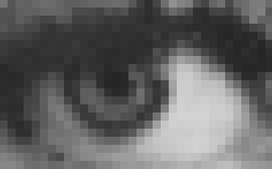
Is that an eye?

When the pixels are sufficiently small, or when they are viewed from sufficiently far away, our human visual system cannot distinguish individual pixels and they blend together into what appears to be a smooth, continuous image.

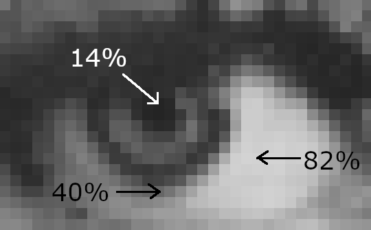
It’s Lena’s left eye! Lena is a commonly-used example of a grayscale raster image

By using colored blocks and a sufficient number of pixels, raster images can represent complex imagery such as people, nature, drawn art, and more. In fact, you are probably already familiar with the versatility of raster images – all modern digital photography produces raster images!

We can better understand the details of raster graphics by ignoring color for the moment and considering black & white, or grayscale, images.

Grayscale

In a grayscale image, each pixel is composed of a single number that represents the amount of black (or white) that appears in that pixel.  The number is sometimes referred to as the intensity, and it can be helpful to think of the intensity as a percentage between 0% and 100%.

Zoomed in view of 3×3 image

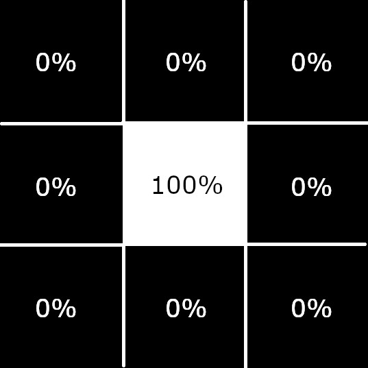
The image above is a zoomed-in view of a image that’s 3 pixels high and 3 pixels wide. This is typically referred to as a 3×3 image (width x height). In this image, all the pixels are either black or white – none are gray.

One way to think of this image is white paper in a dark room. We can illuminate each pixel with white light. Dim white illumination on a pixel would turn it gray. Bright white illumination on the pixel would turn it white. We can quantify the brightness of the illumination as the intensity, where 0% = no light and 100% = bright white light.

This scheme, where increasing intensity produces lighter colors, is known as additive. The image below has been annotated with the additive intensities for each pixel.

3×3 image, with borders between pixels, and annotated with additive intensities for each pixel

Though many interesting images can be created using only black and white pixels that are uniformly square and located on a uniform grid, more realistic detail can be represented when shades of gray are allowed as well.

In the image of Lena’s eye above, 82% points to a near-white pixel, 14% points to a near-black pixel, and 40% points to a mid-tone pixel. So, using varying intensities of black and white between 0% and 100% allows us to clearly represent this eye, which can be discerned even when highly zoomed in.

Color

In a grayscale image, the image is made of pixels that vary in lightness between white and black. Each pixel has a single intensity: the amount of white illumination on a black pixel.

Rather than varying intensity between white and black, which produces shades of gray, we could instead vary between white and a different color. For example, varying intensity between white and red produces shades of pink.

Red-Green-Blue (RGB) images

Full color images are created by combining multiple single color images. When multiple single color images are combined into a full color image, each color is called a separation or channel. In a full color image, each pixel has multiple intensities – one for each channel. The pixel’s color is the combination of each channel’s color at that pixel.

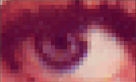
Full color Lena eye

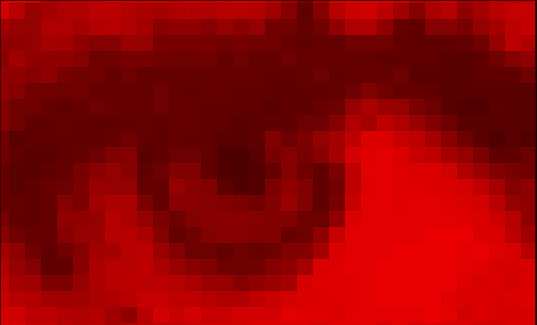
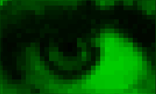
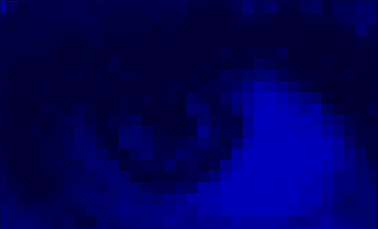
The full color eye above is composed of a red channel, green channel, and blue channel, which are shown below.

Red channel from the full color Lena eye. Note that this is different from a red colorized version of the grayscale image.
Green channel from the full color Lena eye
Blue channel from the full color Lena eye

One aspect of this image that’s immediately noticeable is that each channel is relatively dark on average, yet the full color image is relatively light. That occurs because in the Red-Green-Blue (RGB) scheme, colors are additive – as intensity increases, the amount of light increases, making the image brighter.

The RGB scheme can be interpreted as the red, green, and blue components of a white light that illuminate a white paper in a dark room. For example, if the blue channel’s intensity is 0% for a pixel, it means none of the blue component of white light is illuminating that pixel. If the blue channel’s intensity is 10% for a pixel, it means a little bit of the blue component of white light is illuminating that pixel. If the blue channel’s intensity is 100% for a pixel, it means all of the blue component of white light is illuminating that pixel.

A pixel with intensities 50% red, 50% blue, and 0% green would have a purplish color. Can you think of how to create a white, gray, or yellow pixel?

This website shows how different RGB intensity percentages can create different colors. The table also includes another component, alpha, which is the transparency of the color. 0% is completely opaque, while 100% is completely transparent. Transparency allows background color to mix into the foreground color.

RGB is a common scheme to use because computer screens very commonly are manufactured to emit red, green, and blue light, which combine to create millions of colors. By using RGB data to store image data, the image data translates directly to the display: each pixel on the display just emits red, green, and blue light at the intensity stored in the image’s pixel.

Conclusion

That’s the absolute basics on raster still images! Raster images represent images by describing a uniform grid made of tiny squares called pixels. Each pixel has a color, which is described by one or more intensities.

Raster images are optimal for complex static imagery, such as photography. The pixels allow for arbitrary variation and irregular shapes, which appear throughout our natural world.

Questions? Leave a comment in the comment section below.

The GoF book defines the Factory Method pattern in terms of an ICreator interface that defines a virtual function, CreateIProduct().  The virtual function CreateIProduct() returns a base class, IProduct.  So, classes that derive from ICreator implement CreateIProduct() to return a subclass of IProduct.  In other words, a SubclassOfCreator would create a SubclassOfProduct.

Like the Abstract Factory pattern, this enforces object cohesion – the SubclassOfCreator creates only the types that it can work with.  It also allows for extensibility, because the framework is only providing the ICreator and IProduct interfaces.  The client code will derive from ICreator and IProduct, which eliminates the need for client-specific behaviors in the framework’s code.

Continue reading

Let’s discuss the Abstract Factory pattern to continue our tour of design patterns in C++ .  This is an interesting technique for maintaining coherence between objects, while allowing easy switching or swapping of object sets.  This can be useful for allowing an application to use multiple UI toolkits (Apple vs. Windows), allowing different enemies with different capabilities in a game, using different submodels in a complicated simulation, and much more.

Continue reading

I’m researching image processing techniques for my new job.  I’m finding lots of things that I never took the time to understand, even if I had encountered them.  One of them is color maps.  Color maps are ways to convert a set of scalar values into colors.  They can be used to visualize non-visual data, or enhance visual data.

Continue reading

We’ll start the discussion of design patterns with the object creation patterns.  First up is the Singleton pattern.  Conceptually, this is used when you want exactly one instance of an object.  A common example is a logger.  Sometimes an application wants all its components to log data to the same destination.  So, developers might create a Singleton logger, then all the components can easily get a handle to its instance and use its API.  But the Singleton pattern has significant drawbacks, and there’s usually better methods for handling situations where you want a Singleton.

Continue reading

This is the first in a series of posts I will write about design patterns.

Design patterns in software development have been heavily influenced by the work of Erich Gamma, Richard Helm, Ralph Johnson and John Vlissides, known as the Gang of Four (GoF).  They literally wrote the book on patterns, Design Patterns: Elements of Reusable Object-Oriented Software.  In this book, the authors describe patterns for managing object creation, composing objects into larger structures, and coordinating control flow between objects.  Since publication, other developers have identified and described more patterns in practically every area of software design. Try googling your favorite software topic + “design patterns” to see what kind of patterns other developers have identified and described: android design patterns, embedded design patterns, machine learning design patterns, etc.

It’s very useful to know about the patterns in abstract, even if you don’t know the details of a particular pattern.  As the authors state, knowing the patterns helps developers identify and use the “right” design faster.  Knowing the patterns provides these benefits to the developer:

  1. They describe common problems that occur in software development.  As a developer, especially a new developer, it’s easy to think of every problem as completely unique to the program that you’re writing.  But very often, they are unique only because of poor modeling or simply lack of experience.  Simply knowing common problems can help a developer model a system in terms of those problems, which often reduces the size, number, and complexity of the problems that remain to be solved.
  2. They are considered “best known methods” for solving typical/frequent problems that arise in programming & architecture.  Knowing the “best known method” for solving a problem eliminates a lot of thought, effort, and time devoted to solving it, which reduces the time that a developer must spend on a particular problem.
  3. Knowledge of the patterns simplifies & clarifies communication between developers when talking about a particular problem or solution.  When a developer who is familiar with design patterns hears “I used the singleton pattern on the LogFile class,” the developer immediately knows that (if implemented correctly) there will only be one or zero instances of the LogFile class living in the program at one time.

When to use it

It’s pretty easy to describe when to use a pattern – whenever your program contains the exact problem that is solved by one of the patterns.  They can even be used if your program contains a similar problem to that solved by one of the patterns, but in this case, the implementation of the pattern may need to be modified to fit the particulars of your program.

However, it’s not always obvious your software’s problem(s) can be solved by a GoF pattern.  In other words, the program may be such a mess that it needs to be refactored simply to transform a problem into one that can be solved with a GoF pattern.  Hopefully by learning about the patterns, you’ll be able to recognize non-obvious applications in your own software.


I’ll cover the patterns by subject, and within a subject I’ll try to cover what I feel are the most broadly applicable patterns first.  Stay updated by following me on RSS, linkedin, or twitter (@avitevet)!

Many problems in real life can be represented as optimization problems that are subject to various constraints.  How far can I go without stopping at the gas station if I expect to drive 60% on the highway and 40% in the city?   What’s the most enjoyment I can get with $10 of chocolate bars, given that I want at least one Butterfinger bar but like Snickers twice as much?  How can I achieve the best GPA given my current grades in the classes, each class’s grading system, and that I only have 2 more days to study for finals?

The simplex method is an algorithm for finding a maximal function value given a set of constraints.  We’ll start with a non-trivial example that shows why we need a rigorous method to solve this problem, then move on to a simple example that illustrates most of the main parts of the simplex method.  You’ll learn when to use it, you can check out my cheatsheet, and you can review my code on github!

Continue reading